The creation of an RDF knowledge graph for a particular application commonly involves a pipeline of tools that transform a set of input data sources into an RDF knowledge graph in a process called dataset augmentation. The components of such augmentation pipelines often require extensive configuration to lead to satisfactory results. Thus, non-experts are often unable to use them. We present an efficient supervised algorithm based on genetic programming for learning knowledge graph augmentation pipelines of arbitrary length. Our approach uses multi-expression learning to learn augmentation pipelines able to achieve a high F-measure on the training data. Our evaluation suggests that our approach can efficiently learn a larger class of RDF dataset augmentation tasks than the state of the art while using only a single training example. Even on the most complex augmentation problem we posed, our approach consistently achieves an average F1-measure of 99% in under 500 iterations with an average runtime of 16 seconds.

• Information systems → Entity resolution ; Data cleaning ; Extraction, transformation and loading ; Data exchange; Mediators and data integration; Wrappers (data mining); Deduplication; Geographic information systems; • Computing methodologies → Ontology engineering ; Semantic networks .

Knowledge graphs, Data augmentation, Data integration, Machine learning, Genetic programming, Multi expression programming

ACM Reference Format:

Knowledge graph augmentation encompasses the steps from an initial set of data sources to the creation of a useful knowledge graph for a particular application [26]. For example, the generation of DBpedia¹ demands the mappings of infoboxes to Resource Description Framework (RDF) resources and properties. Large biomedical datasets such as the Linked Cancer Genome Atlas [24] are often the results of the transformation of relational and textual data into RDF including the disambiguation of the terms found in the original dataset. While a plethora of solutions exist for addressing single steps of the knowledge graph augmentation problem (e.g., knowledge extraction [14], link discovery [18], data fusion [15]), there is still a need to combine these solutions with each other as well as with custom dataset transformations to generate the intended data set. Despite a substantial amount of efforts to develop dataset augmentation tasks for specific use cases [1, 5, 10], there are only two frameworks dedicated to facilitating the generation of augmentation tasks, namely DEER [26] and Linked Data Integration Framework (LDIF) [25]. Both frameworks can be configured manually, which requires expert knowledge. They also provide supervised machine learning algorithms, i.e., they can also be operated by non-experts. However, DEER can only operate on a single dataset at a time while LDIF only provides a learning algorithm [3] for its data fusion sub-module SIEVE.

We address these shortcomings by developing an automatic configuration approach (dubbed ADAGIO) for augmentation tasks in the shape of Directed Acyclic Graphs (DAGs) (i.e., with multiple inputs). We implement our approach on top of our own fork² of the DEER framework that supports a plugin system. Moreover, we treat the plugins as black boxes to show the adaptability of our approach in contrast to the state of the art (e.g. LDIF), which has a static pipeline architecture.

The contributions of this paper are summarized as follows:

We present a theoretical framework of RDF dataset augmentation and a classification of DAG-shaped augmentation tasks.

We derive an efficient genotype representation of DAGshaped augmentation tasks for Multi Expression Programming (MEP).

1https://www.dbpedia.org/

2https://github.com/dice-group/deer

43

HT’22, June 28 – July 1, 2022, Barcelona, Spain

Dreßler et al.

We develop various optimizations for our learning algorithm, including a set of semantic genetic operators.

Finally, we evaluate ADAGIO to answer three research questions. In particular, we study the set of optimal hyperparameters of our approach, its performance in comparison to the state of the art and its performance characteristics. Our results show that ADAGIO outperforms the state of the art while being able to learn complex real-world DAG-shaped augmentation tasks with an average F1-measure of 99% in at most 500 generations.

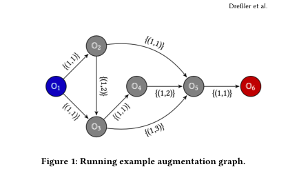
Figure 1: Running example augmentation graph.

The objective of this work is strongly related to the fields of AutoML [7] and On-The-Fly (OTF) Computing [11]. Another closely related notion is that of knowledge graph refinement [22], which is concerned with predictive modelling of certain knowledge graph features.

Genetic Programming (GP) is a subfield of Genetic Algorithm (GA) [17] which originated from the application of a GA in order to evolve computer programs by John Koza[12]. In GP, programs are usually encoded as trees of operations and terminals, but other encodings have also been proposed. For example, Graff et al.[9] use DAGs to encode python programs. Multi Expression Programming (MEP) [6] is a special kind of Genetic Programming [12] that has gained traction in recent years. In particular, MEP has been successfully applied to TSP [19], data prediction [29], software effort estimation [2], on-the-fly hyperparameter optimization for Evolutionary Algorithms [20] and digital circuit design [21]. Semantic genetic operators operate on the semantics of the solution space in contrast to traditional genetic operators, which operate in the encoding space, unaware of the semantics behind traditional bitvector representations. Such semantic genetic operators also have had a lot of attention in recent literature. In particular, [23] uses semantic genetic operators in an NLP context to match sentences. [4, 8] applied semantic genetic operators to symbolic regression problems while other works focus more on advantageous mathematical properties in traditional numerical optimization settings for GP [28].

RDF data augmentation is a problem that greatly differs from use case to use case. For example, [1] considers the automatic extraction of interests from Twitter posts in order to enrich user profiles on the Social Web. On another use case, [5] applies a ranking method to the Youtube tag space in order to enrich datasets on the Linked Open Data (LOD) with links to Youtube videos. To our best knowledge, the only effort directed towards a general framework of RDF dataset augmentation together with an automatic learning approach can be found in [26], where the authors propose a framework and learning algorithm called DEER. We chose to build our approach based on the existing open source software of DEER, where we replaced the simple sequential pipelining approach with a more sophisticated one, based on arranging the enrichment functions in a DAG. In order to better distinguish our approach from the former, we will call atomic enrichment functions which allow for multiple inputs and multiple outputs enrichment operators .

We begin by providing a formal definition of augmentation operators and augmentation graphs. We then show how augmentation tables can be used to evaluate such graphs efficiently. Our learning algorithm then exploits the representation of graphs as multiexpressive augmentation tables to learn augmentation pipelines based on minimal examples.

RDF Dataset. An RDF dataset D is a set of triples {( s , p , o ) ∈ (R ∪B) × R × (R ∪B ∪L)}, where R is the set of all RDF IRI resources, B is the set of all RDF blank nodes and L is the set of all RDF literals. We denote the set of all RDF datasets as D.

Dataset Operators. A function O( n , m ) : Dⁿ⁺¹ →D^m is called a dataset operator . Intuitively, a dataset operator O( n , m ) processes n input datasets using another dataset C as configuration to produce m output datasets. We call n the in-degree and m the out-degree of O( n , m ) and will resort to writing just O when the lack of their specification will incur no loss of generality. Given integers i ∈[1, n ], j ∈[1, m ], we call the i th argument of O( n , m ) and the j th component in the output of O( n , m ) the in-port i and out-port j , respectively. The set of all dataset operators is denoted as O. We specify the following naming scheme for dataset operators: O(0,1) is called a dataset emitter , O(1,0) is called a dataset acceptor , O( n >0, m >0) is called an augmentation operator and O( n ,1) is called a confluent augmentation operator .

Augmentation Graphs. An augmentation graph G = (O, E, L, M) is a directed acyclic labeled multigraph where O ⊆ O is a set of dataset operators, which act as vertices; E ⊆ O² is the set of edges, which represent flow of data; L : E → 2^N×N is the edge labeling function, which defines mappings between dataset operator outports and in-ports for a given edge; and M : O →D is a mapping from vertices to configuration datasets.

O l � �O( n , m ) ∈ O | � �O( n , m ), O^′� ∈ E ∧ n = 1 ∧ m = 0� leaf vertices and O i � O(O r ∪ O l ) inner vertices .

Note that, per definition all root vertices of an augmentation graph must be dataset emitters, all leaf vertices must be dataset acceptors and all inner vertices must be augmentation operators. In

44

HT’22, June 28 – July 1, 2022, Barcelona, Spain

ADAGIO — Automated Data Augmentation of KGs Using MEL

our running example augmentation graph in Figure 1, we coloured all root vertices blue and all leaf vertices red.

The intuition behind L is that, given e = (O1, O2), we need to define which of O1’s out-ports map to which of O2’s in-ports. In other words, an entry of the label multiset l ∈ L( e ) = ( i , j ) establishes a flow of data from O1’s i th out-port to O2’s j th in-port. The label function must not allow multiple mappings to the same in-port of the same dataset operator, which is formally expressed as:

For instance, in our running example in Figure 1, the label set on the edge between O4 and O5 indicates that O4’s first output dataset is the second argument to O5.

To evaluate an augmentation graph, we first obtain the RDF datasets as output of the root vertices in O r . These datasets then flow through the graph as specified by the semantics we associated with the edge set E and the label multiset L. Whenever a dataset operator O( n , m ) ∈ O i has received all its n input datasets, it is evaluated using M(O( n , m )) as its last argument. The flow through the graph continues until eventually all vertices have been evaluated.

Categorization of Augmentation Graphs. We call an augmentation graph G = (O, E, L, M) linear iff |O r | = |O l | = 1 and ∀O1, O2 ∈ O : O1 � O2 there exists at most a single path between O1 and O2; semi-linear iff |O r | = |O l | = 1 and there is a pair of vertices u , v ∈ O, u � v for which there exist multiple paths from u to v ; confluent iff |O r | > 1 ∧|O l | = 1; inherently confluent iff it is confluent and it only contains confluent augmentation operators, i.e., ∀O( n , m ) ∈ O : m = 1; and general otherwise. Note that inherently confluent augmentation graphs correspond to general augmentation graphs without loss of generality³ .

Augmentation Tables. An augmentation table T is a condensed linear representation for inherently confluent augmentation graphs based on column tables [13]. The idea behind this representation is that each row represents one dataset operator. We can go through this table from top to bottom and evaluate the dataset operators which correspond to a row i using only the results of rows 1 to i − 1. Since dataset acceptors produce no output, they are omitted in this representation for the sake of simplicity.

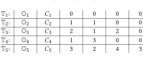
Let G = (O, E, L, M) be an inherently confluent augmentation graph. Moreover, let N (O) � max � n | O( n , m ) ∈ O � denote the maximum in-degree in O. An augmentation table is a table with 3 + N (O) columns and |O| rows, where the first column contains dataset operators, the second column contains configuration datasets and the third column contains the in-degrees of the dataset operators in the first column. The last N (O) columns contain the indices of the rows used as input to the corresponding dataset operator. Given an augmentation table T, we write T i and T i , j to refer to the i th row and the j th column in the i th row of T, respectively. Applying this representation to our running example augmentation graph in Figure 1 gives the augmentation table depicted in Table 1.

The algorithm for the computation of an augmentation table from a given inherently confluent augmentation graph is given

3Any n -ary operator on a set is a finite composition of binary operators [27]

Table 1: Running example augmentation table.

in [13]. In essence, an augmentation table can be easily obtained from the adjacency matrix of a given Directed Acyclic Graph (DAG) G = (V, E) when a fixed indexing bijection ϕ : V →{1, . . . , |O|} of its vertices is provided such that ∀( v , v^′ ) ∈ E : ϕ ( v ) > ϕ ( v^′ ).

To obtain the results of a given augmentation table T, it has to be evaluated from top to bottom. The last result is considered to be the result of the whole table. The evaluation result of a row T i is denoted as T i . For example, the augmentation graph depicted in Table 1 is evaluated as follows:

We call a row within an augmentation table an output row , if it is not used as input to a subsequent row. Note that output rows always correspond to dataset acceptors and that our previous definition of augmentation tables allows for only a single output row, as our augmentation tables must be isomorphic to inherently confluent augmentation graphs.

Multi-Expressive Augmentation Tables. A multi-expressive augmentation table is a generalized augmentation table that has more than one output row . Note that any row ω = T i in a multi-expressive augmentation table can be seen as an output row by just disregarding all rows below ω . Given such a reference output row ω in a multi-expressive augmentation table T we can derive a normal augmentation table T^′ in the following recursive fashion:

(1) We initialize T^′ as an empty augmentation table, L as an empty list and ζ : N → N as a bijective mapping of index numbers that initially only contains the mapping 1 �→ 1.

(2) Given ω = T i , we add ( ω , i ) to the list L

(3) Whenever adding a row T j to L, we recursively add all the row-index pairs ��TT j , 4 , T j ,4� , . . . , �TT j , T j , 3 , T j ,3+T j , 3 �� to L.

(4) We iterate through L’s entries (T k , jk ) ∀ k ∈[1, |L|] in ascending order according to the index jk .

(5) For each entry (T k , jk ) ∈L, we add T k to T^′ and keep track of the mapping from the old row number to the new row number by adding the mapping jk �→ k to ζ .

(6) We then apply our index mapping ζ to the input definition column entries as T x^′ , y � ζ �T x^′ , y � ∀1 ≤ x ∈≤|T^′ |, y ∈ 4, 3 + T^′

� k ,3�

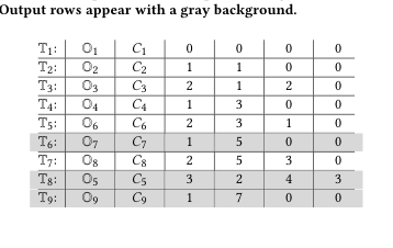
Consider the multi-expressive augmentation table given in Table 2. When we select the 8th row as output reference row, we can

45

HT’22, June 28 – July 1, 2022, Barcelona, Spain

Dreßler et al.

Table 2: Example of a multi-expressive augmentation table. Output rows appear with a gray background.

reconstruct the normal augmentation table in Table 1 by following the algorithm defined above.

The problem under study to find an adequate enrichment graph for a given training example. Since for this work we do not wish to consider multi-objective learning, we restrict ourselves to learning the subclass of inherently confluent enrichment graphs. We will furthermore restrict our study to enrichment graphs where the maximum in-degree of the involved enrichment operators and the number of involved dataset emitters are at most two.

The core of our learning approach is a population-based ( µ + λ ) Multi Expression Programming (MEP) algorithm⁴ that is able to learn the subclass of inherently confluent augmentation graphs. Our population consists of a fixed number µ + λ of multi-expressive augmentation tables that we also call genotypes . All genotypes have a fixed number r of rows. Tournament selection [16] with a tournament size of 3 and a selection probability of 0.75 is applied for determining the mating pool and for selecting the survivors. Additionally, we use 1-elitist selection [17] to avoid a decrease in fitness. Both the offspring and the survivors are subject to mutation. The offspring fraction λ^{µ, mutation probability}^{σand mutation rate} ρ are hyperparameters that need to be determined experimentally. The algorithm will stop when either a perfect solution is found, a maximum number д of generations is exceeded or our convergence detection terminates it.

As the results of RDF dataset augmentation are commonly expected to have a regular structure, we can expect the output dataset to be decomposable into a number of subgraphs that are isomorphic up to a certain error w.r.t. some structural graph similarity measure. We therefore regard the training examples as a list of source Concise Bounded Descriptions (CBDs)^� Ds 1 , . . . , Dsn � ∈D n , n ∈{1, 2} and a single target CBD Dt ∈D of sufficient depth to representatively capture the desired augmentation. This is in accordance with the observation that a single pair of CBDs often suffices for the training of augmentation pipelines [26]. Note our choice to restrict the number of involved dataset emitters to at most two. This restriction does induce loss of generality as a larger number of dataset emitters can be supported by extending some of the formalism and definitions that follow.

4 µ is the population size and λ is the recombination pool size .

In the following, we outline the details of our learning algorithm such as how we compute the initial population, the fitness function we employ and how we use it to evaluate genotypes, as well as a method to speed up learning called genotype compaction and the semantic genetic operators that we use for mutation and recombination.

Algorithm 1: Random generation of multi-expressive augmentation tables.

Population Initialization. The population initialization procedure (see Listing 1) receives a set of prespecified dataset emitters E^⊥ and a corresponding set of configuration datasets C^⊥ as well as the number of rows r it should generate. Initially, the configuration dataset for each of the augmentation operators is the empty dataset. We determine the actual configuration dataset of a given genotype row at evaluation time using heuristic self-configuration .

Heuristic Self-Configuration of Augmentation Operators. Due to the generality of our approach, we will not predefine any augmentation operators. Rather, augmentation operators are black boxes to the learning algorithm, where each augmentation operator expose a generic interfaces for heuristic self-configuration, i.e., a function that can heuristically compute the configuration dataset for the augmentation operator. Formally, let T be a genotype. T i denotes the dataset resulting from the evaluation of a given genotype row T i . The input to the self-configuration procedure consists of the result of all input rows �T i ,4, . . . , T i ,T i , 3 � of T i and the target training dataset Dt .

Fitness Function. Let S( D ), P( D ), O( D ) denote the sets of subjects, predicates and objects⁵ of a given dataset D , respectively. We

5Note that we exclude blank nodes from S( D ) and O( D ).

46

HT’22, June 28 – July 1, 2022, Barcelona, Spain

ADAGIO — Automated Data Augmentation of KGs Using MEL

define the fitness function of our learning algorithm as

where Dr is the resulted dataset from our algorithm, Dt is the target dataset from the training data and F 1 is the F1-measure, F measures similarity in terms of the overlapping IRI resources in subjects, overlapping IRI resources in predicates and overlapping IRI resources and literals in objects as well as overlapping triples. The design of our fitness function is motivated by the two simple observations that (1) augmentation operators seldom modify all components of a given triple at once and (2) generally only the combination of multiple augmentation operators will lead to the generation of a triple as present in the target training dataset. Therefore, we designed our fitness function to detect any incremental improvements towards the end result. In contrast, DEER uses just the F1-measure over the set of triples as fitness function, which completely fails to measure incremental improvements in partial solution quality.

MEP-based Evaluation of Genotypes. As our genotypes are represented as multi-expressive augmentation table T, they correspond to multiple phenotypes. i.e., normal augmentation tables. Therefore, we regard each row in T as a potential output row. The evaluation of T is done row-wise and in a similar way to the evaluation of a normal augmentation table with the notable exception that we apply self-configuration to obtain the configuration dataset.

We compute the fitness for the result of each row using F . The effective phenotype of a given genotype is the normal augmentation table obtained by reconstruction where the fittest row is taken as reference output row. Likewise, we define a genotypes effective fitness as the fitness of its effective phenotype.

Genotype Compaction. The idea of genotype compaction is that we can speedup learning by restructuring genotypes T in a way such that we move the effective phenotype T p of T to the front of the compacted genotype T^′ .

Let |T| denote the number of rows in a given genotype T. Furthermore, let ⊥(T) denote the first one or two rows corresponding to dataset emitters in a given genotype T.

First, we derive the effective genotype T p of T. We define ⊤(T) = T⊥(T). The compacted genotype T^′ is then defined row-wise by Equation 1 where rndrow() means that in this case we generate a new row randomly in a way that is reflected by lines 12 through 19 of Listing 1.

We apply genotype compaction randomly with a probability of 0.5 to the whole population in the beginning of each generation.

To further minimize the size of the compacted genotype, we detect and remove no-op rows , i.e., rows for which the output is identical to one of the inputs. Formally, given a row T i , its input

datasets I = �TT i , 4 , . . . , TT i , 3+T i , 3 � and its output dataset T i , we call T i a no-op row iff ∃ D ∈ I : T i = D .

Subgraph Merging Crossover. The idea behind our subgraph merging crossover is to combine two genotypes T, T^′ in a way that increases the probability of learning a graph where both T and T^′ are part of its effective phenotype. This is motivated by the observation that two well-performing and sufficiently distinct inherently confluent augmentation graphs could be merged into one by redirecting the vertices that have edges to their dataset acceptors to a new vertex with in-degree two.

Let T p , T p^′ be the effective phenotypes of T, T^′ , respectively. We apply this operator only if |⊥(T)| + |⊤(T p )| + |⊤(T p^′ )| ≤ r holds, otherwise we default to the single-point crossover.

The subgraph merging crossover needs to return two child genotypes to guarantee that the population size stays constant. To this end, we first compute both children equally, but then we fill the r −|⊥(T)| + |⊤(T p )| + |⊤(T p^′ )| remaining rows randomly for each child genotype.

If r −|⊥(T)| + |⊤(T p )| + |⊤(T p^′ )| ≥ 1, we will also insert a row that merges the two subgraphs in T p and T p^′ with a probability of 0.25. To this end, we will randomly aquire an augmentation operator with an in-degree of two and set the input columns to the positions of the output rows of T p and T p^′ in the newly created child genotype.

Let O^merge be a randomly chosen augmentation operator with (2,1) in-degree two. Formally, a child genotype T^c is defined row-wise as

Precondition Broadcasting Mutation. The idea of the precondition broadcasting mutation is to define a context-sensitive measure of applicability for augmentation operators. To this end, the augmentation operators need to provide an additional method ⅁, which accepts the same kind of arguments as the self-configuration method. It then returns a real value between 0 and 1, which expresses the applicability of the augmentation operator, given the input and target datasets.

The precondition broadcasting mutation works as follows. When a row T i has been chosen for mutation in a given genotype T, we evaluate T up to T i and obtain the evaluation results of its input dataset(s). Subsequently we broadcast the input dataset(s) together with the target training dataset to the applicability methods ⅁

47

HT’22, June 28 – July 1, 2022, Barcelona, Spain

Dreßler et al.

<!-- Start of picture text --> α = 0 . 0 0 . 9 2 5
2 8
α = 0 . 2
2 8
α = 0 . 4 2 7 2 4
α = 0 . 6 0 . 7
α = 0 . 8 2 6
2 6 α = 1 . 0 2 3
2 5
0 . 5
2 4 2 4 2 2
2 3
0 . 3
2 2 2 2 2 1
0 . 1 2 1
0 . 1 0 . 3 0 . 5 0 . 7 0 . 9 0 . 9 0 . 7 0 . 5 0 . 3 0 . 1 0 . 1 0 . 3 0 . 5 0 . 7 0 . 9 2 0
ρ
σ ρ
σ
StandardDeviation #GenerationsMean
#GenerationsMean
<!-- End of picture text -->

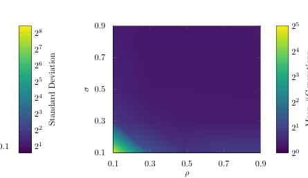
Figure 2: Hyperparameter Optimization Results. The experiment was repeated one thousand times. We measured the average generations to termination and the number of perfect runs. On the right hand side we see a more detailed heat map of the best performing plane on the left.

of all available augmentation operators. After the operators have returned their result, we initialize a roulette wheel selection where the selection probabilities of the roulette wheel are proportional to the relative applicabilities of the operators. Finally, we set T i ,1 to the winner of the roulette wheel.

We chose the name precondition broadcasting for this method, as the input datasets to an augmentation operator can be regarded as its preconditions w.r.t. applicability.

Convergence Detection Mechanism. Our convergence detection mechanism is used to (1) detect convergence of our population and (2) prohibit convergence into a local optima by temporarily adjusting σ and ρ . We keep track of the best fitness value and the standard deviation of fitness values in our generations to detect convergence. We assert convergence if the best fitness value has not changed and the standard deviation of fitness values has been under a certain threshold s min for the last ten generations.

When convergence is detected, we attempt to escape the potential local optima by temporarily setting σ = ρ = 1. In the following generations, we lower them again by multiplication with a constant factor until they reach their initial values. The algorithm finally terminates if, after a fixed number of convergence detections and escape attempts, no perfect solution is found.

Augmentation Operator Setup. We reimplemented the set of augmentation operators used in DEER [26] for the purpose of this evaluation with the notable difference that the linking operator is a binary operator in our implementation⁶ . Additionally, we implemented caching for augmentation operators that rely on external webservices, such as dereferencing or named entity recognition, so that we do not have to unnecessarily query these services a lot of times within our learning loop⁷ . Finally, we introduced a binary merge operator that accepts two datasets and returns their union.

To determine the best set of values for our hyperparameters offspring fraction α = λ^µ,^{mutation probability σand}^{mutation rate ρ,} we used an incrementally explorative method. That is, we ran a series of grid searches on augmentation tasks with increasing difficulty and used our insights from previous runs to fine-tune the next. Due to lack of space, we only report the final grid search results in Figure 2. These results suggest that the best set of hyperparameters are α = 1, σ = 0.5 and ρ = 0.5. It is notable that for these hyperparameters we achieve 100% perfect results despite enabling our convergence detection mechanism. Another interpretation of the data worth mentioning is that the average number of generations to termination is lower for some other settings, but these settings did not achieve a similar number of perfect results.

Research Questions. ( Q 1 ) What is the set of optimal hyperparameters, if any? ( Q 2 ) How does ADAGIO perform compared to the only comparable approach DEER? ( Q 3 ) What are the performance characteristics of ADAGIO when used for DAG-shaped augmentation tasks?

Hardware. All experiments were carried out on a 64-core 2.3 GHz server running OpenJDK 64-Bit Server 1.8.0151 on Ubuntu 16.04.3 LTS. Each experiment was assigned 128 GB RAM.

For this series of experiments, we emulated the 8 original experiments undertaken in [26], using the three original datasets, i.e.,

6This means it is possible to apply instance matching to two input datsets, whereas the linking operator in DEER was unary, requiring another external configuration.

7Please note that this does not introduce bias into our comparison with DEER, since DEER also evaluate each operator only once in every iteration due to its deterministic design based on refinement operators.

48

HT’22, June 28 – July 1, 2022, Barcelona, Spain

ADAGIO — Automated Data Augmentation of KGs Using MEL

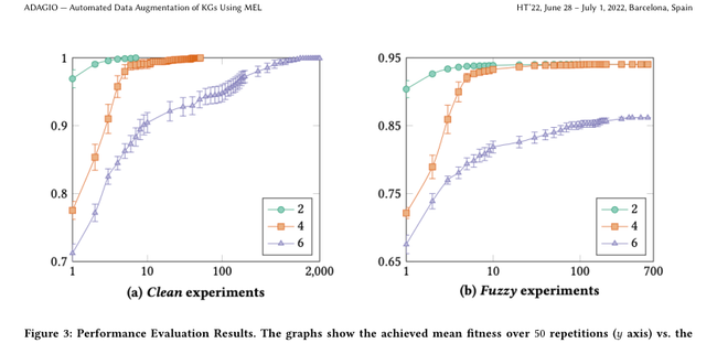
Figure 3: Performance Evaluation Results. The graphs show the achieved mean fitness over 50 repetitions ( y axis) vs. the number of generations on a logarithmic scale ( x axis).

<!-- Start of picture text --> dbo:Town
"1947-0-0" "49610"
"Quakenbrück" ( Ds 1) ( Ds 2) "Quakenbrück"
dbo:producerOf dbo:country
dbr:IslandoftheDead(2000film) dbr:PeterKoper ex:Quakenbrück dbr:Germany
"Peter Koper"@en "52.67722320556640625"
dbr:JohnsHopkinsUniversity "7.9574999809265136719"
"Peter Koper (born 1947) is an ..."
dbr:TimSoutham ( Dt )
dbo:producerOf
dbr:IslandoftheDead(2000film) my:PeterKoper "Quakenbrück"
dbr:Germany
"Peter Koper"@en
ex:Quakenbrück dbo:Town
dbr:ParamountPictures rdf:type
dbr:Baltimore "52.67722320556640625"
"7.9574999809265136719"
dbo:country
dbo:birthPlace rdfs:label
my:name
foaf:name
dbo:director
geo:lat
geo:lat
my:relatedTo
dbo:birthDate dbo:postalCode
rdfs:label
my:relatedTo
dbo:almaMater geo:long
geo:long
rdf:type
my:birthPlace
rdfs:comment
<!-- End of picture text -->

Figure 4: Performance Evaluation Training Data. ( Ds 1 ) shows the CBD used as the first source training dataset, ( Ds 2 ) shows the CBD used as the second source training dataset and ( Dt ) shows the target training dataset, which we generated from ( Ds 1 ) and ( Ds 2 ) using an augmentation graph with 6 augmentation operators.

49

HT’22, June 28 – July 1, 2022, Barcelona, Spain

Dreßler et al.

Table 3: DEER Comparison Results. Reproduced experiments from DEER. tl is the learning time of one execution in seconds, F 1 is the F 1 -measure and max д is the maximum generation after which a perfect solution was found for ADAGIO.

DBpedia⁸ , DrugBank⁹ and Jamendo¹⁰ . We then faithfully recreated the augmentation pipelines in our system. All experiments were repeated 50 times. The results of our comparison are shown in Table 3. ADAGIO constructed a perfect linear augmentation graph in under 4 iterations for all experiments. Moreover, ADAGIO outperformed DEER in terms of learning time in 7 out of 8 experiments with a mean speedup of 6.99. Note that we cannot explain the missing 1% in some of the F1-measure reported in the original DEER paper and that, given the authors methodology, it is most likely that this is due to floating point errors in their F1-measure calculations. ADAGIO was able to parallelize the target augmentation graph for the task MDBpedia^{3, thereby achieving a speedup of 23% compared to the} equivalent linear augmentation graph when applying them to the whole dataset. Altogether, these results suggest that our approach outperforms the current state of the art for learning augmentation pipelines.

We ran two sets of experiments ( clean and fuzzy ) with two realworld datasets extracted from DBpedia¹¹ to measure performance on DAG-shaped augmentation tasks. We obtained one dataset Ds 1 about 2, 230 persons born in Germany and another dataset Ds 2 about 1, 660 towns in Germany. The training data for the experiments was generated using three manually designed augmentation tasks with 2, 4 and 6 augmentation operators for each series of

8 DBpedia is a subset of AdministrativeRegion class instances from the multi-domain knowledge graph DBpedia (https://dbpedia.org).

9 DrugBank is the Linked Data version of the DrugBank database, which is a repository of almost 5000 FDA-approved small molecule and biotech drugs, available at http: //datahub.io/dataset/fu-berlin-drugbank.

10 Jamendo contains a large collection of music related information about artists and recordings

11https://dbpedia.org

experiments, respectively. For the clean experiments, the training data was left untouched, resulting in tasks that ADAGIO is theoretically able to solve perfectly, i.e., with F = 1. For the fuzzy experiments, we randomly altered the training data in a way that the augmentation operators in ADAGIO are not able to solve the tasks perfectly.

For each task, we selected a maximal training example as corresponding CBDs from Ds 1 , Ds 2 and Dt from the training data, for which all components of the augmentation graph contributed to the augmentation in Dt . ADAGIO was then trained on this maximal example using a genotype size of r = 10 and a population size of 30. Figure 4 shows the training data for the the hardest clean task. We measured the performance of ADAGIO by averaging the best fitness found in each generation over a series of 50 repetitions for each task, terminating each task after at most 2, 000 generations. Moreover, we measured run times of our algorithm. We computed 95%-confidence intervals using Student’s t-distribution to account for variance.

The clean results in Figure 3a suggest that our approach solved this task for the two simpler tasks in less than 52 and 7 generations, respectively. Note that this means ADAGIO always found the perfect solution for the simpler tasks. The hardest tasks fitness also grows rapidly over the first 10 generations, reaching an overall average fitness of over 0.99 within a 95% -confidence interval of ±0.6% in under 500 generations . The average runtime reported was 16 seconds for the hardest task .

The fuzzy results in Figure 3b show that our convergence detection is indeed working, as all tasks terminate before the maximum number of 2, 000 generations is reached. Moreover, we see that the solutions of all executions tend to reach the global maximum before termination as the 95%-confidence interval stays at 0% for all generations starting at the 40th, 130th and 366th generation for the 2-, 4- and 6-augmentation operator tasks, respectively.

In this paper, we present ADAGIO, an efficient algorithm based on genetic programming for learning knowledge graph augmentation graphs. We experimentally identified the set of optimal hyperparameters for our algorithm: offspring fraction α = 1.0, mutation probability σ = 0.5 and mutation rate ρ = 0.5, which answers our first research question ( Q 1 ) . To answer ( Q 2 ) , our experiments show that our approach performs at least as well as the previous state of the art. On real-world datasets, ADAGIO reported an average execution time of 16 seconds and a mean solution quality of 99% within a 95%-confidence interval of ±0.6% after 500 generations, thus giving an answer for ( Q 3 ) .

In future work, we will investigate research relating to the automated augmentation of RDF datasets in three directions. (I) We will develop a sound theory of self-configuration heuristics, where we intend to use graph embedding techniques and variations of approximate solutions to the subgraph isomorphism problem. (II) We also intend to extend the class of augmentation graphs for which we investigate learning methods, eventually developing multi-objective algorithms. Such algorithms could be used to automate the provision of RDF knowledge graphs for different types of consumers given the same input datasets, thereby exploiting parallelism. (III)

50

HT’22, June 28 – July 1, 2022, Barcelona, Spain

ADAGIO — Automated Data Augmentation of KGs Using MEL

Finally, we will research methods for improving the scalability of our approach in a big data setting.

This work was supported by the German Research Foundation (DFG) within the Collaborative Research Centre “On-The-Fly Computing“ (GZ: SFB 901/3) under the project number 160364472. This work was also supported by the German Federal Ministry of Economics and Climate Protection (BMWK) project RAKI (GA no. 01MD19012D) and the EU H2020 project KnowGraphs (GA no. 860801).

[1] Fabian Abel, Qi Gao, Geert-Jan Houben, and Ke Tao. 2011. Semantic Enrichment of Twitter Posts for User Profile Construction on the Social Web. In The Semanic Web: Research and Applications , Grigoris Antoniou, Marko Grobelnik, Elena Simperl, Bijan Parsia, Dimitris Plexousakis, Pieter De Leenheer, and Jeff Pan (Eds.). Springer Berlin Heidelberg, Berlin, Heidelberg, 375–389. https://doi.org/ 10.1007/978-3-642-21064-826

[2] Najla Akram, Al-Saati, and Taghreed Riyadh Alreffaee. 2018. Using Multi Expression Programming in Software Effort Estimation. CoRR abs/1805.00090 (2018). https://dblp.org/rec/journals/corr/abs-1805-00090

[3] Volha Bryl and Christian Bizer. 2014. Learning Conflict Resolution Strategies for Cross-Language Wikipedia Data Fusion. In Proceedings of the 23rd International Conference on World Wide Web (Seoul, Korea) (WWW ’14 Companion) . Association for Computing Machinery, New York, NY, USA, 1129–1134. https://doi.org/10. 1145/2567948.2578999

[4] Qi Chen, Bing Xue, Yi Mei, and Mengjie Zhang. 2017. Geometric Semantic Crossover with an Angle-Aware Mating Scheme in Genetic Programming for Symbolic Regression. In EuroGP (Lecture Notes in Computer Science, Vol. 10196) . Springer, 229–245. https://doi.org/10.1007/978-3-319-55696-315

[5] Smitashree Choudhury, John G. Breslin, and Alexandre Passant. 2009. Enrichment and Ranking of the YouTube Tag Space and Integration with the Linked Data Cloud. In The Semantic Web - ISWC 2009 , Abraham Bernstein, David R. Karger, Tom Heath, Lee Feigenbaum, Diana Maynard, Enrico Motta, and Krishnaprasad Thirunarayan (Eds.). Springer Berlin Heidelberg, Berlin, Heidelberg, 747–762. https://doi.org/10.1007/978-3-642-04930-947

[6] Cândida Ferreira. 2001. Gene Expression Programming: A New Adaptive Algorithm for Solving Problems. Complex Systems 13, 2 (2001). https://dblp.org/rec/ journals/compsys/Ferreira01

[7] Matthias Feurer, Aaron Klein, Katharina Eggensperger, Jost Tobias Springenberg, Manuel Blum, and Frank Hutter. 2019. Auto-sklearn: Efficient and Robust Automated Machine Learning . Springer International Publishing, Cham, 113–134. https://doi.org/10.1007/978-3-030-05318-56

Workshops (Berlin, Germany) (EDBT-ICDT ’12) . Association for Computing Machinery, New York, NY, USA, 116–123. https://doi.org/10.1145/2320765.2320803

[16] Brad L. Miller and David E. Goldberg. 1995. Genetic Algorithms, Tournament Selection, and the Effects of Noise. Complex Systems 9, 3 (1995). https://dblp.org/ rec/journals/compsys/MillerG95

[17] Melanie Mitchell. 1998. An introduction to genetic algorithms . MIT Press. https: //dblp.org/rec/books/daglib/0019083

[18] Markus Nentwig, Michael Hartung, Axel-Cyrille Ngonga Ngomo, and Erhard Rahm. 2017. A survey of current Link Discovery frameworks. Semantic Web 8, 3 (2017), 419–436. https://doi.org/10.3233/SW-150210

[19] Mihai Oltean and Dumitru Dumitrescu. 2015. Evolving TSP heuristics using Multi Expression Programming. CoRR abs/1509.02459 (2015). https://dblp.org/ rec/journals/corr/OlteanD15

[20] Mihai Oltean and Crina Groşan. 2003. Evolving Evolutionary Algorithms Using Multi Expression Programming. In Advances in Artificial Life , Wolfgang Banzhaf, Jens Ziegler, Thomas Christaller, Peter Dittrich, and Jan T. Kim (Eds.). Springer Berlin Heidelberg, Berlin, Heidelberg, 651–658.

[21] Mihai Oltean and Crina Grosan. 2004. Evolving Digital Circuits using Multi Expression Programming. In Evolvable Hardware . IEEE, IEEE Computer Society, 87–90. https://doi.org/10.1109/EH.2004.1310814

[22] Heiko Paulheim. 2017. Knowledge graph refinement: A survey of approaches and evaluation methods. Semantic Web 8, 3 (2017), 489–508. https://doi.org/10. 3233/SW-160218

[23] Dunlu Peng, Shaohong Wu, and Cong Liu. 2019. MPSC: A Multiple-Perspective Semantics-Crossover Model for Matching Sentences. IEEE Access 7 (2019), 61320– 61330. https://doi.org/10.1109/ACCESS.2019.2915937

[24] Muhammad Saleem, Maulik R Kamdar, Aftab Iqbal, Shanmukha Sampath, Helena F Deus, and Axel-Cyrille Ngonga Ngomo. 2014. Big linked cancer data: Integrating linked tcga and pubmed. Web Semantics: Science, Services and Agents on the World Wide Web 27 (2014), 34–41. https://doi.org/10.1016/j.websem.2014.07.004

[25] Andreas Schultz, Andrea Matteini, Robert Isele, Christian Bizer, and Christian Becker. 2011. LDIF -Linked Data Integration Framework. In Proceedings of the Second International Conference on Consuming Linked Data - Volume 782 (Bonn, Germany) (COLD’11) . CEUR-WS.org, Aachen, DEU, 125–130.

[26] Mohamed Ahmed Sherif, Axel-Cyrille Ngonga Ngomo, and Jens Lehmann. 2015. Automating RDF Dataset Transformation and Enrichment. In The Semantic Web. Latest Advances and New Domains , Fabien Gandon, Marta Sabou, Harald Sack, Claudia d’Amato, Philippe Cudré-Mauroux, and Antoine Zimmermann (Eds.). Springer International Publishing, Cham, 371–387.

[27] Wacław Sierpiński. 1945. Sur les fonctions de plusieurs variables. Fundamenta Mathematicae 33, 1 (1945), 169–173. http://eudml.org/doc/213088

[28] Ranyart Rodrigo Suárez, Mario Graff, and Juan J. Flores. 2015. Semantic Crossover Operator for GP based on the Second Partial Derivative of the Error Function. Research in Computing Science 94 (2015), 87–96. https://dblp.org/rec/journals/ rcs/SuarezGF15

[29] Qingke Zhang, Bo Yang, Lin Wang, and Jianzhang Jiang. 2013. An improved multi-expression programming algorithm applied in function discovery and data prediction. IJICT 5, 3/4 (2013), 218–233. https://doi.org/10.1504/IJICT.2013.054952

[8] Stefan Forstenlechner, David Fagan, Miguel Nicolau, and Michael O’Neill. 2017. Semantics-Based Crossover for Program Synthesis in Genetic Programming. In Artificial Evolution (Lecture Notes in Computer Science, Vol. 10764) . Springer, 58–71. https://doi.org/10.1007/978-3-319-78133-45

[9] M. Graff, E. S. Tellez, S. Miranda-Jiménez, and H. J. Escalante. 2016. EvoDAG: A semantic Genetic Programming Python library. In 2016 IEEE International Autumn Meeting on Power, Electronics and Computing (ROPEC) . 1–6. https: //doi.org/10.1109/ROPEC.2016.7830633

[10] Souleiman Hasan, Edward Curry, Mauricio Banduk, and Sean O’Riain. 2011. Toward situation awareness for the semantic sensor web: Complex event processing with dynamic linked data enrichment, In Proceedings of the 4th International Conference on Semantic Sensor Networks-Volume 839. Semantic Sensor Networks , 69–82.

[11] Holger Karl, Dennis Kundisch, Friedhelm Meyer auf der Heide, and Heike Wehrheim. 2019. A Case for a New IT Ecosystem: On-The-Fly Computing. Business & Information Systems Engineering 62, 6 (Dec 2019), 467–481. https: //doi.org/10.1007/s12599-019-00627-x

[12] John R Koza. 1990. Genetic programming: A paradigm for genetically breeding populations of computer programs to solve problems . Vol. 34. Stanford University, Department of Computer Science Stanford, CA.

[13] Vladimír Kvasnièka and Jiøí Pospíchal. 1998. Simple Implementation of Genetic Programming by Column Tables. In Soft Computing in Engineering Design and Manufacturing , P. K. Chawdhry, R. Roy, and R. K. Pant (Eds.). Springer London, London, 48–56. https://doi.org/10.1007/978-1-4471-0427-86

[14] Jose Lazaro Martinez-Rodriguez, Aidan Hogan, and Ivan López-Arévalo. 2020. Information extraction meets the Semantic Web: A survey. Semantic Web 11 (2020), 255–335. https://doi.org/10.3233/sw-180333

[15] Pablo N. Mendes, Hannes Mühleisen, and Christian Bizer. 2012. Sieve: Linked Data Quality Assessment and Fusion. In Proceedings of the 2012 Joint EDBT/ICDT

51

PDF page 2.

PDF page 3.

PDF page 4.

PDF page 6.

PDF page 7.